Naked Word: Nationalities of World Language

Part One: Feature Engineering -- Syntactic and Ad-hoc

Steps: 1. Loading all essays in their raw txt form

def load_data_multi(root):
    all_docs = []
    for path, sub, filen in os.walk(root):
        for f in filen:
            if f == '.DS_Store':
                continue
            doc_path = path+'/'+f
            all_docs.append(doc_path)
    print len(all_docs)
    df = pd.DataFrame({'path':all_docs, 'doc_id':range(1,len(all_docs)+1)})
    df['author_code'] = df['path'].apply(lambda x: x.split('/')[-1])
    df['essay_content'] = df['path'].apply(read_file)
    df['label'] = df['author_code'].apply(lambda x: x.split('_')[1])
    return df

2. Using spaCy to extract the following ad-hoc features:

import spacy
spc_nlp = spacy.load('en')

• unique_lemma: Count of unique lemmatized words in an essay

df_0['unique_lemma'] = df_0['essay_content'].apply(lambda x: len(set([token.lemma_ for token in \ spc_nlp(x.decode('utf-8')) if token.is_punct==False])))

• avg_stc_length: Count of average sentence length (how many words are there in a sentence) of an essay

df_0['avg_stc_length'] = df_0['essay_content'].apply(lambda x: np.mean([len(s) for s in \ spc_nlp(x.decode('utf-8')).sents]))

• total_stc: Count of sentences in an essay

df_0['total_stc'] = df_0['essay_content'].apply(lambda x: len([s for s in spc_nlp(x.decode('utf-8')).sents]))

NOTE I did some basic explortory data analysis on the three generated features. And there are some fascinating findings: 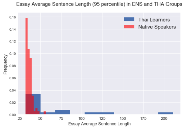The plot above shows that compared to native speakers, learners from Thailand tend to write more much longer sentences. This may be explained by the fact that in Thai(the language) script, full-stop doesn't exist. Therefore, the learners brought this habit to their L2 (English) writing See source code here

3. Tagging, Parsing and Bag of Words It's intuitive to think that for native language identification(NLI), capturing features that reflecting syntactic characteristics is necessary. Therefore I generated POS tags and dependent tree elements for each essay in my corpus. For these features, I again used spaCy considering the tagging speed it offers compare to NLTK. The tagging convention of spaCy is following OntoNotes 5 version of the Penn Treebank tag set. The columns are shown below: - DT_pos: Part-of-Speech tags for each word in an essay

df_0['DT_pos'] = df_0['essay_content'].apply(lambda x: [' '.join([token.pos_ for token in spc_nlp(s.text)]) for s in spc_nlp(x.decode('utf-8')).sents])

Example result:

It was important for me because it allowed me to take time off and travel to Japan.
PROPN VERB ADJ ADP PRON ADP PRON VERB PRON PART VERB NOUN PART CCONJ VERB ADP PROPN PUNCT

• DT_archs: Dependent tree element labeling for each word in an essay

df_0['DT_archs'] = df_0['essay_content'].apply(lambda x: [' '.join([token.dep_ for token in spc_nlp(s.text)]) for s in spc_nlp(x.decode('utf-8')).sents])

Example result:

It was important for me because it allowed me to take time off and travel to Japan.
nsubj ROOT acomp prep pobj mark nsubj advcl nsubj aux ccomp dobj prt cc conj prep pobj punct

DT_pos and DT_archs are the base features for other syntactic features that captures more detailed characteristics of one's writing style:

DT_pos based

• POS_adjv_repeat_rate: the portion of repeated adjectives and adverbs in an essay's overall vocabulary

df_0['POS_adjv_body'] = df_0['essay_content'].apply(lambda x: [token.text.lower() for token in \ spc_nlp(x.decode('utf-8')) if (token.dep_=='amod')|(token.dep_=='advmod')])

df_0['POS_adjv_repeat_rate'] = df_0['POS_adjv_body'].apply(lambda x: len([k for k, v in dict(Counter(x)).iteritems() if v>1])*1./len(x))

• POS_adjv_repeat_cnt: total number of repeated adjectives and adverbs in an essay

df_0['POS_adjv_repeat_cnt'] = df_0['POS_adjv_body'].apply(lambda x: sum([v for k, v in dict(Counter(x)).iteritems() if v>1]))

DT_archs based

• DT_max_dp_cnts: list of max child-word count of each sentence for an essay

df_0['DT_max_dp_cnts'] = df_0['essay_content'].apply(lambda x: [max([len([c for c in token.children]) \
for token in spc_nlp(s.text)]) \
for s in spc_nlp(x.decode('utf-8')).sents])

Based on this feature, several statistics can be calculated on the list for each essay. For example, I can calculate the standard deviation of max child-word counts of each sentence:

df_2['DT_max_dp_cnts_std'] = df_2['DT_max_dp_cnts'].apply(lambda x: np.std(x))

• DT_ROOT_idx: list of positions of the ROOT word in each sentence (see definition of ROOT word here)

df_0['DT_ROOT_idx'] = df_0['DT_archs'].apply(lambda x: [[i for i,e in enumerate(s.split(' ')) if e=='ROOT'][0] for s in x])

• DT_pass_cnt: list of passive words in each sentence in an essay

df_0['DT_pass_cnt'] = df_0['DT_archs'].apply(lambda x: [len([dep for dep in s.split(' ') if dep[-4:]=='pass']) for s in x])

• DT_mark_cnt: list of mark words in each sentence in an essay (see definition of mark word here)

df_0['DT_mark_cnt'] = df_0['DT_archs'].apply(lambda x: [len([dep for dep in s.split(' ') if dep=='mark']) for s in x])

Similarly, a couple of more numeric features can be calculated based on features above:

df_2['DT_ROOT_idx_mean'] = df_2['DT_ROOT_idx'].apply(lambda x: np.mean(x))
df_2['DT_pass_cnt_sum'] = df_2['DT_pass_cnt'].apply(lambda x: np.sum(x))
df_2['DT_mark_cnt_sum'] = df_2['DT_mark_cnt'].apply(lambda x: np.sum(x))

Bag-of-Words (BOW) term frequency matrix has been a very common way to represent a text body with numeric values. However, in the case of NLI, simply transform the original text body of an essay into a term frequency matrix may not suit the text classification task well, given the fact that the model needs to generalize writing style characteristics instead of the actual content of the text bodies in each class. Therefore, I decided to use the idea of BOW and generate term frequency matrix based on the "syntactic-version" of the text body. In many previous academic works, this approach was mentioned as POS n-gram. - DT_pos_join: converting feature DT_pos into one string of pos tags of an essay

df_0['DT_pos_join'] = df_0['DT_pos'].apply(lambda x: ' '.join(x))

• DT_archs_join: converting feature DT_archs into one string of dependent tree tags of an essay

df_0['DT_archs_join'] = df_0['DT_archs'].apply(lambda x: ' '.join(x))

• DT_insent_pos_ngram: same as feature DT_pos_join, but only generate ngram terms within sentence boundary

from nltk import ngrams
def tag_sent_gram(s, n):
    result = []
    n_grams = ngrams(s.split(' '), n)
    for grams in n_grams:
        result.append('_'.join(grams))
    return result


def loop_body(body, n):
    result = []
    for sent in body:
        result.append(tag_sent_gram(sent, n))
    return ' '.join(sum(result, []))

n = 4
df_0['DT_insent_pos_ngram'] = df_0['DT_pos'].apply(lambda x: pwk.loop_body(x, n))

• DT_insent_arch_ngram: same as feature DT_archs_join, but only generate ngram terms within sentence boundary

n = 3
df_0['DT_insent_arch_ngram'] = df_0['DT_archs'].apply(lambda x: pwk.loop_body(x, n))

To transform a syntactic BOW feature into term frequency matrix, below is an example:

X = df_0['DT_pos_join']
y = df_0['label']
X_train, X_test, y_train, y_test = train_test_split(X, y, train_size=0.8)

vectorizer = TfidfVectorizer(lowercase=True, ngram_range=(3,3)).fit(X_train)
X_train_dtm = vectorizer.transform(X_train)
X_test_dtm = vectorizer.transform(X_test)